I always wanted to get my hands dirty with image processing, and the other day I was talking with a friend who works on Restricted Boltzmann Machines (RBMs). The topic sounded very fascinating to me and, after all, I had to start from somewhere… so I decided to implement my own version of a RBM in python. I chose this path, rather than using one of the available codes in the internet (python, C++) or the scikit implementation, because I felt it would give me a deeper understanding of RBMs.

For a very basic introduction of RBMs I recommend Edwin Chen’s blogpost. For the math part I found A. Fischer and C. Igel paper extremely useful. For the tuning of the parameters and training monitoring I followed the guidelines from A Practical Guide to Training Restricted Boltzmann Machines by G. Hinton.

The code is available on my RBM Github repository and I will not post it here. The implementation is vectorized with numpy arrays and so runs in parallel on the CPU in a decent amount of time. Here I will show only the results from my experiments. If you are interested in a short introduction and summary of the math you can also look at the end of this post.

First experiments: visualizing reconstruction and weights representations

I first tested the code by training my RBM on the 60000 handwritten digits of the MNIST dataset (28x28 pixel images). I started with a fairly small RBM with only 10 hidden units. Before training I convert each image in the dataset in black and white, i.e., pixels can only have binary values (0 for white, 1 for black). To monitor the learning progress of an RBM we can plot, for each hidden units, the values of the weights. In particular, since each hidden unit is connected to all the visible (input) units, we can create an image of 28x28 pixels representing the weights.

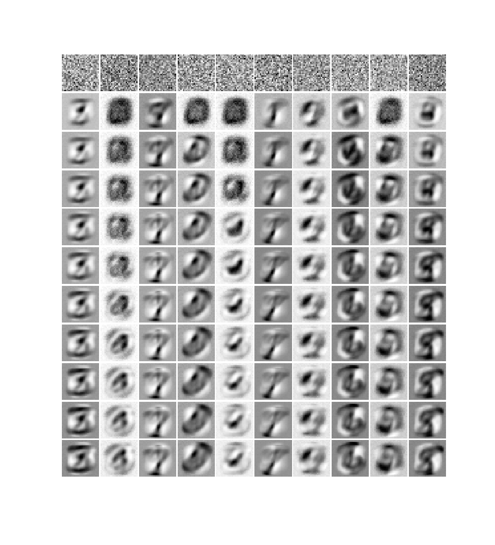
In Figure 2 I show the image representation of the weights for each hidden unit (columns) as the learning progresses at each epoch (rows). Already after the first epoch the RBM has learned interesting features from the data set. We also see that some units train faster than others and start to train at later epochs. We can also try to visualize the reconstruction of the original training images. This is shown in Figure 3: the first column represents samples from the MNIST dataset; the second column is the reconstruction of the image from the trained RBM (after one gibbs sampling step); the subsequent ten images in each row represent the hidden unit weights. On top of each hidden unit I also printed the probability that the unit is activated and I colored the border in red for units which have an appreciable probability of being activated.

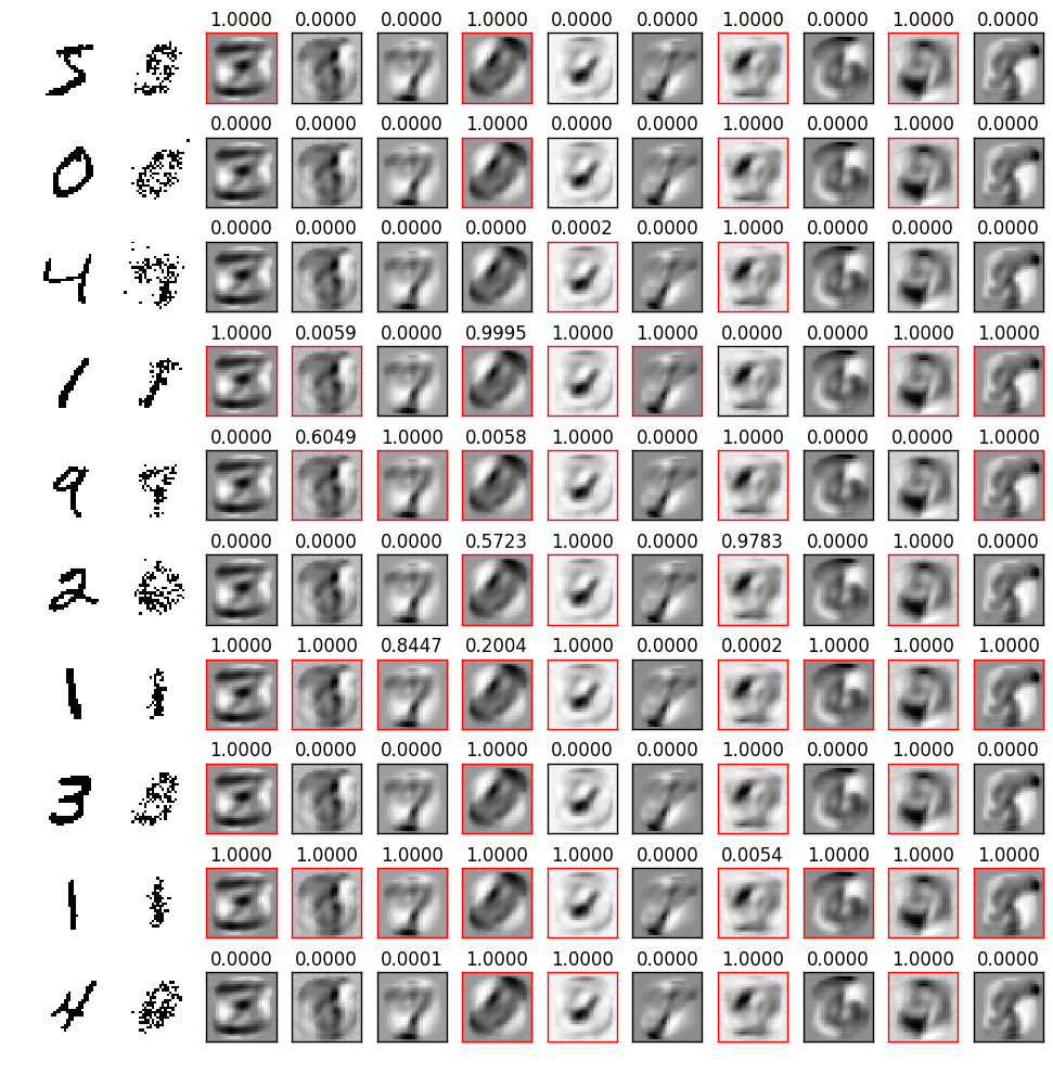
Each one of the above reconstructions represent one sample from the distribution learned by the RBM. What we could do to get a better reconstuction is to draw many samples given the same input and then average them together. I show results obtained in this way in Figure 4, where in the first row are the input images, and in the second row the reconstructions.

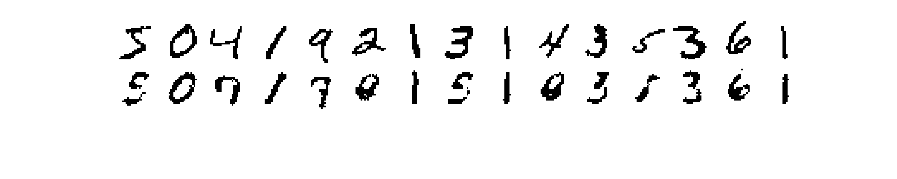
The results now look much better, although there’s still room for improvement.

Large RBM: featuring the strokes

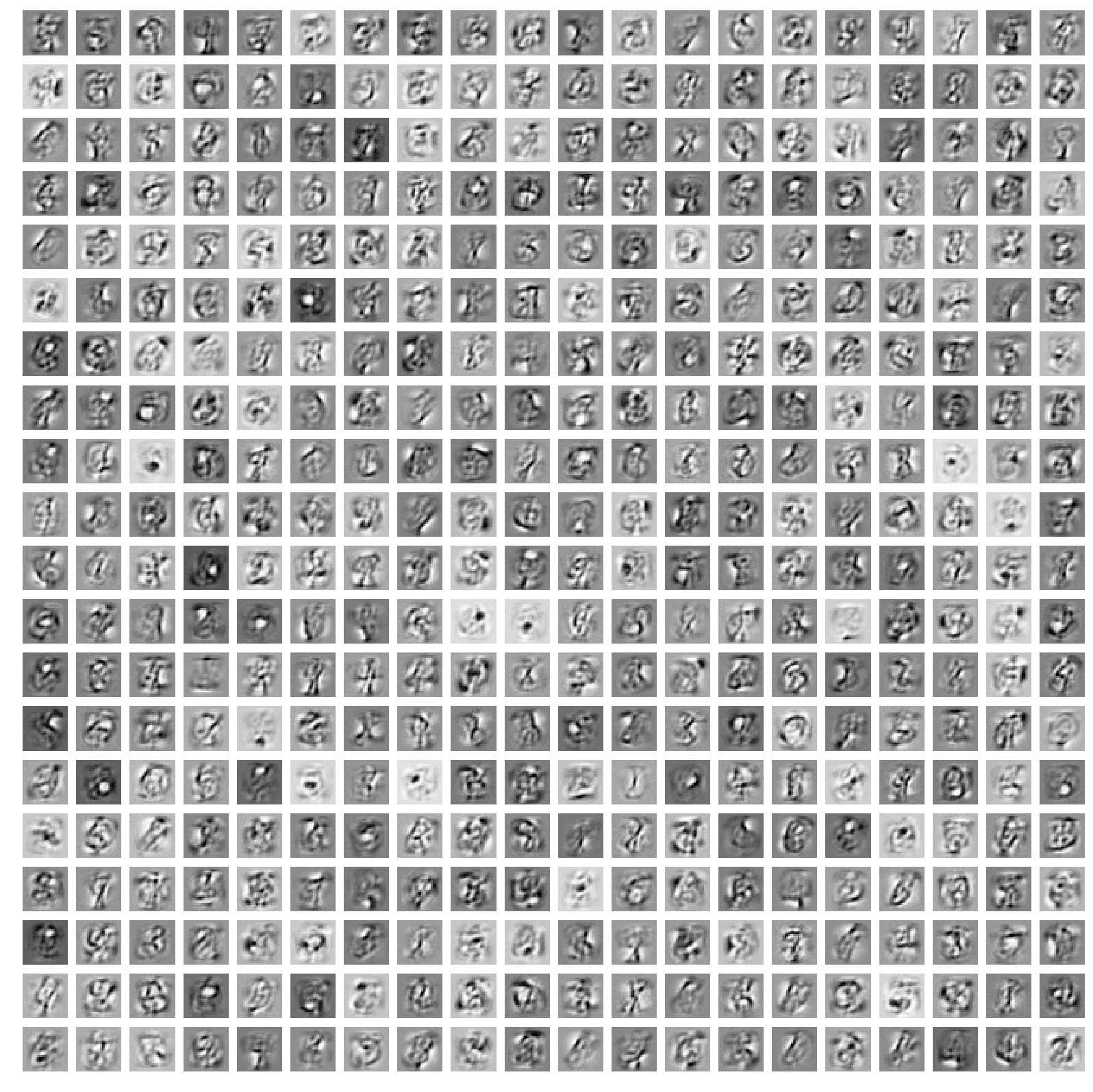
The features learned from the small RBM (Figure 2) resemble the digits in the training dataset very closely, and the reconstructions don’t look too bad. However we can try to do better with a larger model, and if we train a larger RBM, the features learned will look more like the “strokes” of a pen. With 400 hidden units, the weights representations look like in Figure 5: each hidden unit learns a specific trait of the training images.

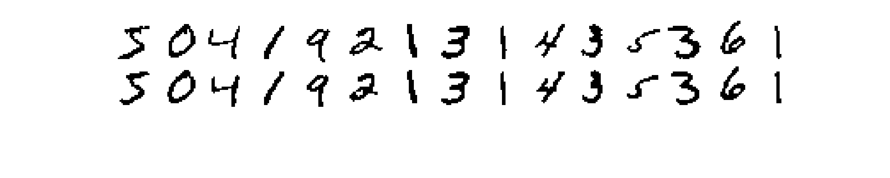
In Figure 6 I show also how this large RBM can reconstruct the training images (I use the same technique I used in Figure 4).

Daydreaming

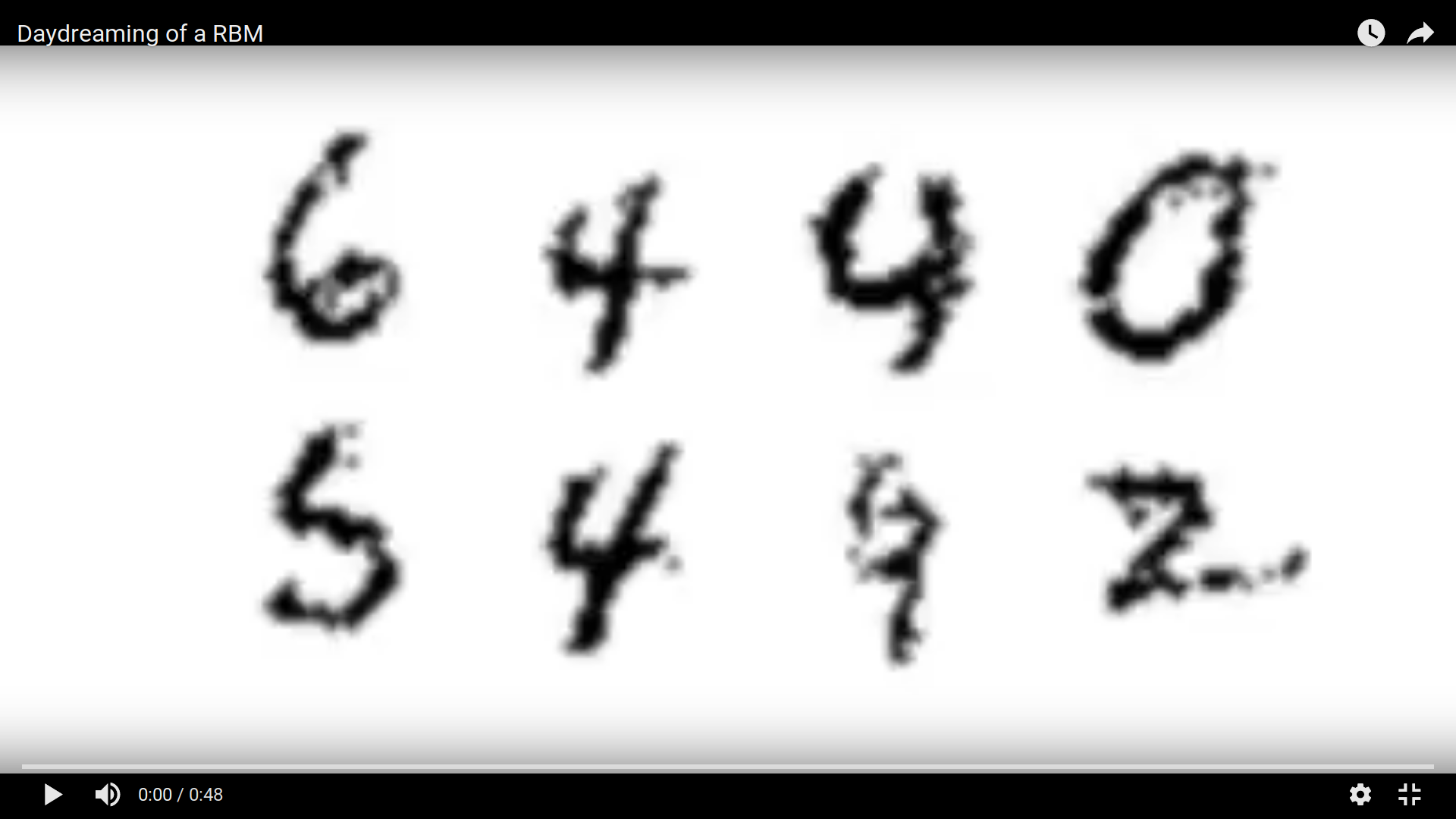
The results for the large RBMs are very very good!!! We can reproduce the training images almost perfectly and it is almost impossible to distinguish between original and reconstructed samples. Unfortunately, training an RBM with 400 hidden units it’s very time expensive (the figures above are generate after only 3 epochs of training). It turns out that I could get pretty decent results with 100 hidden units. In particular with this last medium-size RBM I have been able to generate a “dreaming” video which you can find below (and the gif at the beginning of this post). The video has been obtained by giving some input digits to the trained RBM and then successively sampling from the conditional distributions up to 1000 Gibbs sampling steps.

RBM math and intuition

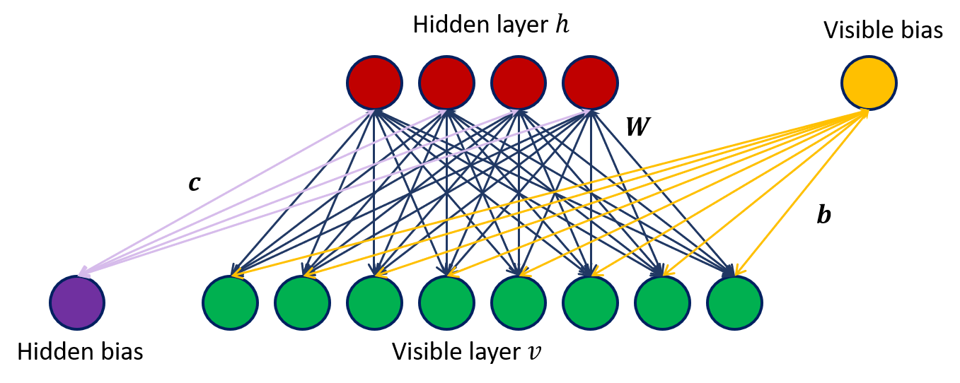
A restricted Boltzmann machine is an energy-based probabilistic model. One has two sets of random variables, the visible variables $v$ and the hidden variables $h$. From a graph point of view we can represent a RBM as in Figure 1, where the green layer represents the visible variables $v$ and the red layer the hidden units $h$. From the above figure is clear where the term “restricted” comes from: the hidden variables are conditionally independent given the visible ones and the visible variables are conditionally independent given the hidden ones (no connections between hidden-hidden and visible-visible units). In other words, given $n_h$ hidden variables and $n_v$ visible variables,

$$P(h|v) = \prod_{j=1}^{n_h}P(h_j|v) \quad\text{and}\quad P(v|h) = \prod_{i=1}^{n_v}P(v_i|h).$$

The joint probability distribution between $v$ and $h$ is defined as

$$P(v,h) = \frac{e^{-E(v,h)}}{\sum_{h,v}e^{-E(v,h)}} = \frac{e^{-E(v,h)}}{Z},$$

where in the last equality we have defined the partition function $Z$, and $E(v,h)$ is the energy associated with a configuration of $h$ and $v$. The energy can be written as

$$E(v,h) = -c^Th - b^Tv - v^TWh,$$

where $c\in\mathbb{R}^{n_h}$ ($b\in\mathbb{R}^{n_v}$) is a vector representing the weights associated to the edges connecting the hidden (visible) units with the bias unit and $W\in\mathbb{R}^{n_v\times n_h}$ is the weights matrix representing the factors associated with the edges connecting hidden and visible units.

Maximizing the likelihood

When we train the RBM we want to maximize the probability $P(v^t)$ of a training data $v^t$ with respect to the parameters $\theta = {b,c,W}$. We can turn this into a minimization problem of the marginal log-likelihood

$$\begin{align} \mathcal{L}^t(\theta) =& {\rm \log} \left[P(v^t)\right]={\rm\log}\left[\sum_hP(v^t,h)\right] \notag \\ =& {\rm\log}\left[\sum_h e^{-E(v^t,h)}\right] - {\rm\log}\left[\sum_{h,v}e^{-E(v,h)}\right]. \end{align}$$

Notice how the second term (coming from the partition function) now does not depend on the observation $v^t$. We can find the gradient and then use simple gradient descent to tune the parameters and maximize $P(v^t)$. However, because of the second term in the above equation (which is a sum over all possible configurations of $h$ and $v$), the log-likelihood is intractable. This is also clear from the gradient of $\mathcal{L}^t(\theta)$ which is given by

$$\begin{align} \nabla_\theta\mathcal{L^t}(\theta) =& -\frac{\sum_h e^{-E(v^t,h)}\frac{\partial E(v^t,h)}{\partial\theta}}{\sum_h e^{-E(v^t,h)}} + \frac{\sum_{h,v} e^{-E(v,h)}\frac{\partial E(v,h)}{\partial\theta}}{\sum_{h,v} e^{-E(v,h)}} \notag \\ =& -\mathbb{E}_{P(h|v^t)}\left[\frac{\partial E(v^t,h)}{\partial\theta}\right] + \mathbb{E}_{P(v,h)}\left[\frac{\partial E(v,h)}{\partial\theta}\right]. \end{align}$$

Contrastive Divergence and conditional distributions

From the above formula we see that in order to evaluate the gradient of the marginal log-likelihood, we need the expectation of the derivative of the energy. While we can obtain the first expectation by sampling only on $h$, for the second we would need to sample on both $h$ and $v$. While this is possible with Gibbs sampling, the problem is still computationally intractable as we would need to draw a large amount of samples for $v$ and $h$. We can avoid this by still making use of Gibbs sampling, but replacing the expectation value by a point estimate at $v=\tilde{v},h=\tilde{h}$. This procedure is also called Contrastive Divergence, which can be summarized as:

• start with $v=v^t$,
• sample $h$ from $P(h|v=v^t)$,
• sample $\tilde{v}$ from $P(v=\tilde{v}|h)$,
• finally sample $\tilde{h}$ from $P(h=\tilde{h}|v=\tilde{v})$.

For the above procedure we need the conditional probabilities. These are easy to find, and for example one has

$$P(h|v) = \frac{P(v,h)}{P(v)} = \frac{e^{c^Th + v^TWh}}{\sum_h e^{c^Th + v^TWh}}.$$

Since $h_j={0,1}\ \forall j=1,…,n_h$, for a single hidden variable we have

$$P(h_j = 1|v) = \frac{e^{c_j + \sum_iv_iW_{ij}}}{1 + e^{c_j + \sum_iv_iW_{ij}}} = \sigma\left(c_j + \sum_iv_iW_{ij}\right),$$

where $\sigma(x)=1 / (1 + e^{-x})$ is the sigmoid function. Since we assum the single hidden units to be conditionally independent from each other, we then have

$$P(h|v) = \prod_{j=1}^{n_h} \sigma\left(c_j + \sum_iv_iW_{ij}\right),$$

and equivalently

$$P(v|h) = \prod_{i=1}^{n_v} \sigma\left(b_i + \sum_jW_{ij}h_j\right).$$

Derivatives of the energy

The last ingredient we need are the derivatives of the energy with respect to the model parameters $\theta={b,c,W}$, which I summarise below:

$$\begin{align} \frac{\partial E(v,h)}{\partial W} = vh^T \quad,\quad\frac{\partial E(v,h)}{\partial b} = v \quad,\quad\frac{\partial E(v,h)}{\partial c}= h. \end{align}$$

The gradients of the marginal log-likelihood are then calculated via

$$\begin{align} \nabla_W\mathcal{L}(\theta) = \mathbb{E}_{P(h|v^t)}\left[v^th^T\right] - \mathbb{E}_{P(v,h)}\left[vh^T\right]= \langle h^T\rangle v^t - \langle vh^T\rangle \end{align}$$ $$\begin{align} \nabla_b\mathcal{L}(\theta) = \mathbb{E}_{P(h|v^t)}\left[v^t\right] - \mathbb{E}_{P(v,h)}\left[v\right]= v^t - \langle v\rangle \end{align}$$ $$\begin{align} \nabla_c\mathcal{L}(\theta) = \mathbb{E}_{P(h|v^t)}\left[h\right] - \mathbb{E}_{P(v,h)}\left[h\right]= \langle h^t\rangle - \langle h\rangle \end{align}$$

The weights and biases can then be updated iteratively with gradient descent using the general formula

$$\begin{align} \theta^{(new)} = \theta^{(old)} - \alpha\nabla_\theta\mathcal{L}(\theta^{(old)})\ \end{align}$$

where $\alpha$ is the learning rate.