All the code can be found here.

The travelling salesman problem is a combinatorial optimization problem. Wikipedia has a decent statement of the problem:

• "Given a list of cities and the distances between each pair of cities, what is the shortest possible route that visits each city exactly once and returns to the origin city?".

Of course, this is a simplification of a real-world problem where, for example, we would also have other constraints such as time and money. We will deal with additional constraints later and for the moment let’s start simple.

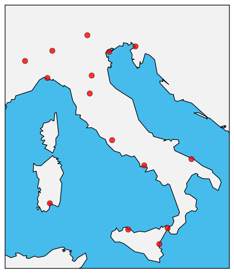
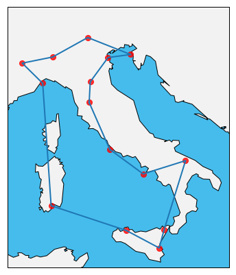
Suppose we want to go on vacation in Italy and visit some of its cities. However, we can only take a couple of weeks of vacation, and so reducing the time we travel between cities (as opposed to the time we spend visiting them) is extremely important. Suppose these cities are the ones represented with red dots in Figure 1. It is sensible to also assume that, if we travel with planes, the travel time between two cities should be roughly proportional to the distance between the two, i.e., $t\propto d$. Then, the problem of minimizing the travel time is basically the same as minimizing the total distance between cities we travel in our trip (path).

Now, we have many possible paths connecting all these cities (the number of paths grows factorially with the number of cities), and so we need some efficient way to explore the configuration space (the space of all the possible paths).

There’s a lot of approaches that one can use to solve this problem (more or less efficiently, see https://en.wikipedia.org/wiki/Travelling_salesman_problem). Here I will focus on simulated annealing. The algorithm is inspired by physical systems, where the crystalline structure of a block of material can be manipulated by heating and successive controlled cooling of the system. The crystalline structure of a material affects its internal energy, and so using annealing, one can drive the energy of the system to a minimum (in our case the energy will be some function of the total travel distance and we will try do drive this function to a minimum).

Simulated Annealing

In particular, I will use a stochastic approach, where we randomly move between states of the configuration space with a probability proportional to a Boltzmann factor $e^{-1/T_k}$, where $T_k$ is the “temperature” of the system after $k$ iterations performed by the algorithm. Let’s call {$c_i$} (${i=1,…,N}$) the set of N cities, and $s_{ij}$ the segment between city $c_i$ and city $c_j$. The steps one has to follow are very simple:

• Randomly connect all the cities and calculate the total length of the path $L_0$ obtained in this way as: $$ L_0 = \sum_{j>i=1}^N s_{ij} $$
• For $k=1$ until convergence, or a finite amount of iterations, perform the following steps:
  • Change the path by, for example, switching two of the cities in the path, and calculate the new length of the path $L_k$.
  • If $L_k<L_{k-1}$ then accept the new path as the best solution. If $L_k>L_{k-1}$, accept $L_k$ as new path with probability proportional to $e^{-\Delta L/T_k}$, where $$ \Delta L = L_k - L_{k-1} $$

In order to simulate annealing, the temperature $T_k$ must decrease with increasing $k$. For example, one could define a schedule like $T_k = c^kT_0,$ where $c$ is a constant which regulates the change in temperature at each step, e. g., $c=0.999$ and $T_0$ is the initial temperature.

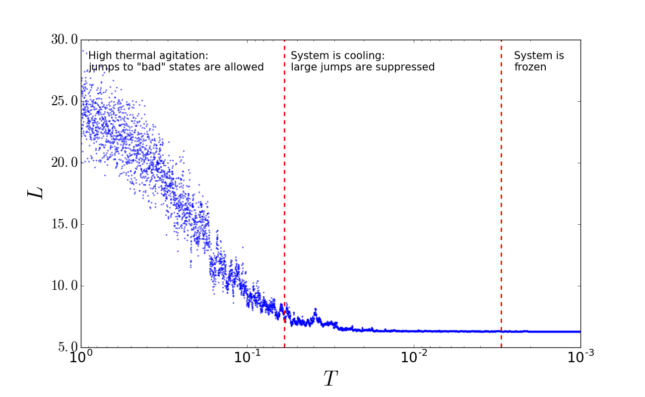
The first iterative step described above has the effect of driving the system towards the shortest path (minimization of the length of the path), while the second step allows for jumps to worse solutions (prevents getting stuck in local minima), with a probability which decreases as the system cools down. This allows for the exploration of large areas of the configuration space at higher temperatures, but lets the system reach a stable state as the temperature decreases.

If we were to plot the length of the best path as a function of the temperature during the annealing schedule, we would obtain something like Figure 2.

So far we just focused on the length of the trip which, as we assumed, is proportional to the trip’s time. In reality we would also be concerned about the amount of money we are going to spend. To take into account the price, we need to add another constraint to our optimization problem. To do so we can modify the function we have to minimize by adding another term to it, i.e.,

where $L$ is again the length of the path and $P$ is the total price of the given path. $J$ is the total cost function. The parameter $\alpha$ regulates how much weight we give to either length or price. For example, setting $\alpha=1$ means we care only about the length of the path, while if $\alpha=0$ we are going to minimize only the price of the path.

Note taht for the function to have any meaning, we will need to normalize both L and P so that they have comparable scales. We can do so by finding the minimum and maximum values for each pair of cities for both distance and price and normalize with respect to this two values (see code below).

Python implementation

Data preparation

So, let’s follow the above steps and try to find the shortest path with the lowest price between the cities in Figure 1. The coordinates of these cities are saved in a file called italy_cities.csv, and are expressed in degrees.minutes. The prices are in a file called italy_prices.csv. While the prices file contains already the prices between any two cities, for the distances we need to create a look-up table: from the coordinates, x and y, we will calculate the distances between any two cities. The code to do this is the following:

# Import libraries
import pandas as pd
import numpy as np

# Read data, create x and y coordinate variables and 
# N which is the total number of cities
df = pd.read_csv("datasets/italy_cities.csv")
N = len(df)
x = np.array(df['Lon'])
y = np.array(df['Lat'])
print(df.head())

$\qquad$> Name Lat Lon
$\qquad$>0 Bologna 44.30 11.21
$\qquad$>1 Cagliari 39.15 9.03
$\qquad$>2 Catania 37.30 15.05
$\qquad$>3 Florence 43.47 11.15
$\qquad$>4 Messina 38.11 15.33

# Now create the lookup-table for the distances
# Extract cities names
cities = df['Name'].values
# Preallocate look-up table
dtable = [[0.0 for c in cities] for c in cities]
# Calculate distances
for i, ci in enumerate(cities):
    for j, cj in enumerate(cities):
        delta_lon = df.loc[df['Name'] == ci, 'Lon'].values - df.loc[df['Name'] == cj, 'Lon'].values
        delta_lat = df.loc[df['Name'] == ci, 'Lat'].values - df.loc[df['Name'] == cj, 'Lat'].values
        dtable[i][j] = float(np.sqrt(delta_lon**2 + delta_lat**2))

# Now we normalize all the distances from 0 to 1
dmax = np.max(dtable)
dmin = np.min(dtable)
dtable = [[(x - dmin) / (dmax - dmin) for x in r] for r in dtable]

For the prices we just need to read in the file and normalize them between 0 and 1 (as well as creating the prices look-up table):

df = pd.read_csv('datasets/italy_prices.csv')
df['price'] = df['price'].apply(lambda x: (x - df['price'].min())/(df['price'].max() - df['price'].min()))
print(df.head(5))

$\qquad$> cityA cityB dist
$\qquad$> 0 Bologna Cagliari 0.474299
$\qquad$> 1 Bologna Catania 0.712602
$\qquad$> 2 Bologna Florence 0.000000
$\qquad$> 3 Bologna Messina 0.657968
$\qquad$> 4 Bologna Milano 0.147987

# Create mapping city-id to setup prices table
mapping = {}
imapping = {}
for idcity,cname in enumerate(cities):
    # mapping: name -> id
    mapping[cname] = idcity
    # inverse mapping: id -> name
    imapping[idcity] = cname
    
# Build price look-up table
ptable = [[0.0 for c in cities] for c in cities]
for i,row in df.iterrows():
    ptable[mapping[row['cityA']]][mapping[row['cityB']]] = row['price']
    ptable[mapping[row['cityB']]][mapping[row['cityA']]] = row['price']

Tracking configurations

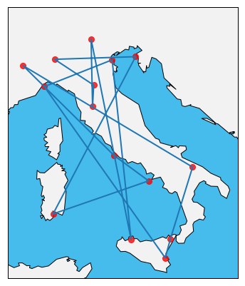
We have to find a way to keep track of the configurations for the paths. Each configuration can be thought as a list of integer numbers, where the integer numbers represent the id of the cities. In particular, we can use the mapping dictionary we defined in the code above to assign an integer id to each city. So, a list like s = [0,3,5,0] will indicate that the path s starts from city with id = 0, passes trough cities with id = 3 and id = 5 in this order, and goes back to the initial city with id = 0. Following this structure, we can create a first random path that we will use as initial state for our simulated annealing schedule. To do so we first create a list containing the N ids of the cities and then we shuffle it randomly. Since we want our path to be closed (i.e. the last city must be the one were we started our trip), we also need to append the id of the first city in the shuffled list to the list end:

# Set seed for reproducibility of the results
np.random.seed(0)
# Initialize state (path)
s = np.arange(N)
np.random.shuffle(s)
# Append first city id to end of path (we need a closed path!)
s = np.append(s,s[0])
print(s)
print([imapping[idc] for idc in s])

$\qquad$>[ 1 6 8 9 14 4 2 13 10 7 11 3 0 5 12 1]
$\qquad$>['Cagliari', 'Napoli', 'Rome', 'Torino', 'Bari',
$\qquad$> 'Messina', 'Catania', 'Genova', 'Venice',
$\qquad$> 'Palermo', 'Trento', 'Florence', >'Bologna',
$\qquad$> 'Milano', 'Trieste', 'Cagliari']

The cost function

To calculate the cost (which takes into account both total price and total length) of a certain configuration s, we can define a function get_cost which calculates $J = \alpha L + (1-\alpha)P$:

# Cost function: inputs are price and distance look-up tables,
# the configuration s, the mixing parameter alpha and the total
# number of cities N
def get_cost(dtable, ptable, alpha, s, N):
    L = 0.0
    P = 0.0
    for i in range(N):
        # Calculate length and price components
        L += dtable[s[i]][s[i+1]]
        P += ptable[s[i]][s[i+1]]
    # Return cost 
    return alpha * L + (1. - alpha) * P

The cost $J$ of the initial random guess can be obtained simply calling this function. In addition, we can also get either the total price or the total distance only by selecting the appropriate value of the mixing parameter $\alpha$:

# Get total cost using a balanced combination of price/length (alpha = 0.5)
alpha = 0.5
total_cost = get_cost(dtable, ptable, alpha, s, N)
print('Total (balanced) cost: %6.4f' %total_cost)
# Get total price using alpha = 0.0
alpha = 0.0
total_cost = get_cost(dtable, ptable, alpha, s, N)
print('Total price: %6.4f' %total_cost)
# Get total distance using alpha = 1.0
alpha = 1.0
total_cost = get_cost(dtable, ptable, alpha, s, N)
print('Total distance: %6.4f' %total_cost)

$\qquad$>Total (balanced) cost: 7.3254
$\qquad$>Total price: 7.8486
$\qquad$>Total distance: 6.8022

Annealing function

We can then implement the annealing procedure outlined in the introduction in a function called anneal. The input parameters will have to be the initial path s and the price and distance look-up tables, ptable and dtable, respectively. Finally, we will also need to input the initial temperature T0 of the annealing schedule and the maximum number of iterations to be performed.

# Inputs are price and distance look-up tables, the mixing parameter alpha,
# the configuration s (a list containing the cities ids in the order of the path),
# the total number of cities N, the initial annealing temperature and the maximum 
# number of iterations to be performed
def anneal(dtable, ptable, alpha, s, N, T0=1.0, iter_max=10000, verbose=True):
    # Counters to keep track of accepted/rejected moves and path length
    acc = 0        
    rej = 0
    J = get_cost(dtable, ptable, alpha, s, N)
    if verbose:
        print('Initial guess length: %7.4f' % l)
    # Array to keep track of the cost as we iterate
    Jarr = [J]
    # Set initial temperature
    T = T0
    if verbose:
        print('Initial temperature: %7.4f' % T0)
    # Initiate iterative steps
    for i in range(1,iter_max+1):
        # Annealing (reduce temperature, cool down with steps)
        # Here we decrease the temperature every 100 steps
        if i % 100 == 0:
            T = 0.999 * T
        # Generate two random indices and switch them (switch cities)
        # We keep first and last cities fixed (note they are also the same
        # since the path must be closed)
        j,k = np.random.randint(low=1,high=N,size=2)
        s_new = np.copy(s)
        s_new[j] = s[k]
        s_new[k] = s[j]
        # Calculate length of new state (path)
        Jnew = get_cost(dtable, ptable, alpha, s_new, N)
        deltaJ = Jnew - J
        # Accept the move if new path is shorter than previous one
        if deltaJ <= 0.0:
            s = np.copy(s_new)
            J = Jnew
            acc += 1
        # If new path is larger than previous, accept the move with probability
        # proportional to the Boltzmann factor
        elif deltaJ > 0.0:
            u = np.random.uniform()
            if u < np.exp( - deltaJ / T):
                s = np.copy(s_new)
                J = Jnew
                acc += 1
            else:
                rej += 1
        # Every 100 steps record the cost
        if i % 100 == 0:
            Jarr.append(J)
    
    # Return final configuration s, list keeping track of the cost,
    # final temperature T and number of accepted and rejected moves
    return s, Jarr, T, acc, rej

The anneal function returns the final optimal (at least we hope it is the optimal one) configuration s, a list Jarr of the total cost at every 100 steps of the annealing schedule, the final temperature T and the number of accepted and rejected moves.

Finding the shortest path

We can now try to run the above function with our initial random guess s and, for simplicity, let us set $\alpha=1.0$, meaning we just want to optimize the path s with respect to the distance only:

# Set seed for reproducibility of the results
np.random.seed(721)
# Set parameters
alpha = 1.0       # Mixing parameter 
T0 = 1.0          # Initial temperature
iter_max = 500000 # Number of iterations
# Simulate annealing
s, Jarr, T, accepted, rejected = anneal(dtable, ptable, alpha, s, N, T0, iter_max, verbose=True)
print('Accepted moves: %d' % accepted)
print('Rejected moves: %d' % rejected)
print('Final temperature: %7.4f' % T)
print('Final length after optimization: %7.4f' % Jarr[-1])

$\qquad$>Initial guess length: 6.8022
$\qquad$>Initial temperature: 1.0000
$\qquad$>Accepted moves: 141842
$\qquad$>Rejected moves: 358158
$\qquad$>Final temperature: 0.0067
$\qquad$>Final length after optimization: 3.0766

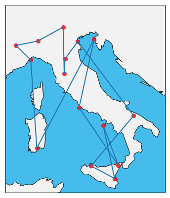
The final length after the optimization is much smaller than the one of our first random guess. To have a better idea if the final path makes sense or not, we can visualize it on a map. The optimal path found is shown in Figure 4.

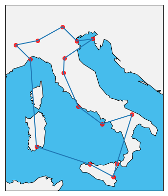
The path found by the annealing procedure looks pretty good, however, how do we know this is really the global optimum of the configuration space? In fact, as we will see later, the path shown in Figure 4, although very close to the global minimum, is only a local optimum. There isn’t really a good way to know if the optimum we find is local or global. It is not guaranteed we end up in a global minumum. A way to alleviate this problem is to run many annealing schedules starting from different random initial configurations and then combine the results in some way to determine the global optimum. For example, one could run the annealing schedule for 10 times and then select the configuration which gives the minimum distance among the ensemble of the 10 annealing schedules. Doing so we obtain:

# Set seed for reproducibility of the results
np.random.seed(0)
# Here we perform simulated annealing 10 times and select as optimal solution
# the one which gives the lowest path
s_best = None
Jbest = None
for i in range(10):
    s = np.arange(N)
    np.random.shuffle(s)
    s = np.append(s,s[0])
    if s_best is None:
        s_best = np.copy(s)
    if Jbest is None:
        Jbest = get_cost(dtable, ptable, alpha, s, N)
    # Set parameters
    alpha = 1.0       # Mixing parameter 
    T0 = 1.0          # Initial temperature
    iter_max = 500000 # Number of iterations
    # Optimize with annealing
    s, Jarr, T, accepted, rejected = anneal(dtable, ptable, alpha, s, N, T0, iter_max, verbose=False)
    # Check if this solution is better than the previous one
    if Jarr[-1] < Jbest:
        Jbest = Jarr[-1]
        s_best = np.copy(s)
print('Length of the optimal path: %7.4f' % Jbest)

$\qquad$>Length of the optimal path: 3.0757

The best path is a bit shorter than the one we found previously and is shown in the above figure.

Finding the shortest (length) and cheaper (price) path

We can now set $alpha=0.5$ and try to optimize both respect to the price and length. We can again run the annealing schedule for 10 times and keep track of the best result. The path which optimizes both price and length is shown in Figure 6.

Scaling up

The example of the italian cities is not that computationally expensive. The situation gets much more complicated and interesting when we increase the number of cities we consider. We can obtain a list of cities and relative coordinates by querying Wikipedia’s database. I used the Wikidata Query system with

SELECT ?item ?itemLabel ?coord ?pop ?countryLabel ?continentLabel
WHERE {
  ?item wdt:P31 wd:Q515 .
  ?item wdt:P625 ?coord .
  ?item wdt:P1082 ?pop .
  ?item wdt:P17 ?country .
  ?country wdt:P30 ?continent
  FILTER(?pop > 1000000)
  SERVICE wikibase:label { bd:serviceParam wikibase:language "[AUTO_LANGUAGE],en". }
}

to query all the cities in the world with more than 1 Million population. The coordinates are given as a geometric point, so I had to import the dataset in python and format the coordinates properly. The cleaned dataset can be found here . The query returns 236 cities, however there’s some duplicates and in practice we have 189 unique cities. Using the simulated annealing functions shown above I optimized for the shortest path’s length. The result of one random annealing schedule is shown in the gif below.

C++ implementation

Since running the python code for a large number of cities and for multiple annealing schedule is quite slow, I also implemented the get_cost and anneal functions in C++. I wrapped C++ functions using pybind11 so that I could import and use them within python. The C++ code with the relative makefile code are just posted below (or you can check out all the code here).

lib_anneal.cpp

// Include pybind headers
#include <pybind11/pybind11.h>
#include <pybind11/stl.h>
#include <pybind11/complex.h>

// headers
#include <vector>
#include <math.h>
#include <random>
#include <iostream>
#include <tuple>

// Function to calculate the cost given two constraints and the mixing parameter
double get_cost(std::vector<std::vector<double>> const &dtable, std::vector<std::vector<double>> const &ptable,
   std::vector<int> const &s, double const &alpha, std::vector<int>::size_type const &N){
   double L = 0.0;
   double P = 0.0;
   #pragma omp parallel for reduction(+: L,P)
   for (std::vector<int>::size_type i = 0; i < N; i++){
      // Calculate length and price components
      if (alpha != 0.0d)
         L += dtable[s[i]][s[i+1]];
      if (alpha != 1.0d)
         P += ptable[s[i]][s[i+1]];
   }
   return alpha * L + (1.0d - alpha) * P;
}

// Annealing schedule to optimize the path between cities at coordinates x and y
void anneal(std::vector<std::vector<double>> const &dtable,
   std::vector<std::vector<double>> const &ptable, double const &alpha,
   std::vector<int>::size_type const &N, std::vector<int> &s, double const &T0, int const &iter_max,
   int const &seed, bool const &verbose, int &acc, int &rej, double &T,
   std::vector<double> &l_arr){

   // Initialize random generators
   std::mt19937 _rng;
   _rng.seed(seed);
   std::uniform_int_distribution<int> _uniform_int(1, N-1); //exclude first and last cities which should also be the same
   std::uniform_real_distribution<double> _uniform_real(0.0d, 1.0d);
   // Preallocate l_arr
   l_arr.reserve(std::ceil((double) iter_max / 10.0d));
   // Temp snew vector
   std::vector<int> snew;
   // Reset counters
   acc = 0; rej = 0;
   // Get initial cost for the random configuration
   double l = get_cost(dtable, ptable, s, alpha, N);
   if (verbose)
      std::cout << "Initial guess length: " << l << '\n';
   l_arr.push_back(l);
   // Set temperature
   T = T0;
   if (verbose)
      std::cout << "Initial temperature: " << T << '\n';
      // Initiate iterative steps
   for (int i = 1; i != iter_max+1; i++){
      // Annealing (reduce temperature, cool down with steps)
      // Here we decrease the temperature every 100 steps
      if (i % 100 == 0)
         T = 0.999 * T;
      // Generate two random indices and switch them (switch cities)
      std::vector<double>::size_type j = _uniform_int(_rng);
      std::vector<double>::size_type k = _uniform_int(_rng);
      snew = s;
      snew[j] = s[k];
      snew[k] = s[j];
      // Calculate cost of new configuration
      double lnew = get_cost(dtable, ptable, snew, alpha, N);
      double deltal = lnew - l;
      // Accept the move if new path is shorter than previous one
      if (deltal <= 0.0d){
          s = snew;
          l = lnew;
          acc += 1;
      } else {
      // If new path is larger than previous, accept the move with probability
      // proportional to the Boltzmann factor
         double u = _uniform_real(_rng);
         if (u < std::exp( - deltal / T)){
            s = snew;
            l = lnew;
            acc += 1;
         } else {
            rej += 1;
         }
      }
      if (i % 10 == 0)
         l_arr.push_back(l);
   }

   return;
}


// Python bindings
namespace py = pybind11;
PYBIND11_MODULE(lib_anneal, m) {
   m.doc() = "LibAnneal";
   // anneal function for Python; inputs are:
   // * dtable: distance look-up table (list of lists)
   // * ptable: price look-up table (list of lists)
   // * alpha: mixing parameter
   // * s: initial configuration (list)
   // * N: number of cities
   // * T0: initial temperature
   // * iter_max: maximum number of iterations
   // * seed: random seed for the random generators
   // * verbose: switch for text output while running
   m.def("anneal", [](std::vector<std::vector<double>> const &dtable,
         std::vector<std::vector<double>> const &ptable, double const &alpha,
          std::vector<int> &s, std::vector<int>::size_type const &N, double const &T0,
         int const &iter_max, int const &seed, bool const &verbose){
            int acc, rej;
            double T;
            std::vector<double> l_arr;
            anneal(dtable,ptable,alpha,N,s,T0,iter_max,seed,verbose,acc,rej,T,l_arr);
            return std::make_tuple(s, l_arr, T, acc, rej);
      });
}

makefile

OBJS = lib_anneal.o

CPU_CC = g++
CPU_BINDFLAGS = -O3 -Wall -shared -fopenmp -std=c++11 -fPIC `python3 -m pybind11 --includes`

lib_anneal : $(OBJS)
	$(CPU_CC) $(CPU_BINDFLAGS) $(OBJS) -o lib_anneal`python3-config --extension-suffix`

lib_anneal.o: 
	$(CPU_CC) $(CPU_BINDFLAGS) -c lib_anneal.cpp

clean:
	rm *.so *.o *.gch

The newly created package can be imported in python using import lib_anneal as lann in python (the .so file created using the makefile must be in the same directory of the python code, or you can just add the path to the package using sys.path.append("path/to/lib_anneal/")). Then we just have to replace the string

s, Jarr, T, accepted, rejected = anneal(dtable, ptable, alpha, s, N, T0, iter_max, verbose=False)

with

s, Jarr, T, accepted, rejected = lann.anneal(dtable, ptable, alpha, s, N, T0, iter_max, seed, True).

The C++ code runs fast enough that I can perform a full annealing schedule (1M iterations) for 189 cities in less than 4 seconds on my machine (Intel(R) Core(TM) i7-6700HQ CPU @ 2.60GHz).